L'entropie différentielle est un concept de la théorie de l'information qui étend le concept de l'entropie de Shannon aux lois de probabilités continues.
Pour une variable aléatoire X avec une distribution de probabilité f et définie sur un ensemble
X
{\displaystyle \mathbb {X} }
h (X )[ 1] (p243) :
h
(
X
)
=
−
∫
X
f
(
x
)
ln
f
(
x
)
d
x
.
{\displaystyle h(X)=-\int _{\mathbb {X} }f(x)\ln f(x)\,\mathrm {d} x.}
Pour les lois de probabilité qui n'ont pas d'expression explicite pour leur densité, mais dont on connait la fonction quantile Q (p )h (Q )Q (p )[ 2] (pp54–59)
h
(
Q
)
=
∫
0
1
ln
Q
′
(
p
)
d
p
.
{\displaystyle h(Q)=\int _{0}^{1}\ln Q'(p)\,\mathrm {d} p.}
Pour un couple de variables aléatoires (X , Y ) de loi jointe f (x ,y )X sachant Y vaut :
h
(
X
|
Y
)
=
−
∫
X
∫
Y
f
(
x
,
y
)
ln
f
(
x
|
y
)
d
x
d
y
.
{\displaystyle h(X|Y)=-\int _{\mathbb {X} }\int _{\mathbb {Y} }f(x,y)\ln f(x|y)\,\mathrm {d} x\mathrm {d} y.}
∀
(
a
,
c
)
∈
R
∗
×
R
,
h
(
a
X
+
c
)
=
h
(
X
)
+
ln
(
|
a
|
)
{\displaystyle \forall (a,c)\in \mathbb {R} ^{*}\times \mathbb {R} ,h(aX+c)=h(X)+\ln(|a|)}
L'entropie différentielle d'une loi continue peut être négative, contrairement à celle d'une loi discrète.
Majoration : Soit X une variable aléatoire continue de variance Var(X ) . Alors on a
h
(
X
)
⩽
1
2
ln
(
2
π
e
V
a
r
(
X
)
)
,
{\displaystyle h(X)\leqslant {\frac {1}{2}}\ln(2\pi \mathrm {e} \mathrm {Var} (X)),}
avec égalité si et seulement si X suit une loi normale[ 1] (p254) .
L'entropie différentielle donne une borne inférieure à l'espérance d'un estimateur . Pour toute variable aléatoire X et un estimateur
X
^
{\displaystyle {\widehat {X}}}
[ 1]
E
[
(
X
−
X
^
)
2
]
≥
1
2
π
e
e
2
h
(
X
)
{\displaystyle \mathbb {E} [(X-{\widehat {X}})^{2}]\geq {\frac {1}{2\pi {\rm {e}}}}{\rm {e}}^{2h(X)}}
avec égalité si et seulement si
X
{\displaystyle X}
X
^
{\displaystyle {\widehat {X}}}
X .
Dans le tableau qui suit,
Γ
(
x
)
=
∫
0
∞
e
−
t
t
x
−
1
d
t
{\textstyle \Gamma (x)=\int _{0}^{\infty }{\rm {e}}^{-t}t^{x-1}{\rm {d}}t}
fonction gamma ,
ψ
(
x
)
=
d
d
x
ln
Γ
(
x
)
=
Γ
′
(
x
)
Γ
(
x
)
{\textstyle \psi (x)={\frac {\rm {d}}{{\rm {d}}x}}\ln \Gamma (x)={\frac {\Gamma '(x)}{\Gamma (x)}}}
fonction digamma ,
B
(
p
,
q
)
=
Γ
(
p
)
Γ
(
q
)
Γ
(
p
+
q
)
{\textstyle \mathrm {B} (p,q)={\frac {\Gamma (p)\Gamma (q)}{\Gamma (p+q)}}}
fonction bêta , et γ constante d'Euler-Mascheroni .
Table d'entropies différentielles de lois usuelles[ 3] (pp120–122) .
Distribution
Fonction de distribution de probabilités
Entropie
Loi uniforme continue
f
(
x
)
=
1
b
−
a
1
1
[
a
,
b
]
{\displaystyle f(x)={\frac {1}{b-a}}1\!\!1_{[a,b]}}
ln
(
b
−
a
)
{\displaystyle \ln(b-a)\,}
Loi normale
f
(
x
)
=
1
2
π
σ
2
exp
(
−
(
x
−
μ
)
2
2
σ
2
)
{\displaystyle f(x)={\frac {1}{\sqrt {2\pi \sigma ^{2}}}}\exp \left(-{\frac {(x-\mu )^{2}}{2\sigma ^{2}}}\right)}
ln
(
σ
2
π
e
)
{\displaystyle \ln \left(\sigma {\sqrt {2\pi \,{\rm {e}}}}\right)}
Loi exponentielle
f
(
x
)
=
λ
exp
(
−
λ
x
)
{\displaystyle f(x)=\lambda \exp \left(-\lambda x\right)}
1
−
ln
λ
{\displaystyle 1-\ln \lambda \,}
Loi de Cauchy
f
(
x
)
=
λ
π
1
λ
2
+
x
2
{\displaystyle f(x)={\frac {\lambda }{\pi }}{\frac {1}{\lambda ^{2}+x^{2}}}}
ln
(
4
π
λ
)
{\displaystyle \ln(4\pi \lambda )\,}
Loi du χ²
f
(
x
)
=
1
2
n
/
2
σ
n
Γ
(
n
/
2
)
x
n
2
−
1
exp
(
−
x
2
σ
2
)
{\displaystyle f(x)={\frac {1}{2^{n/2}\sigma ^{n}\Gamma (n/2)}}x^{{\frac {n}{2}}-1}\exp \left(-{\frac {x}{2\sigma ^{2}}}\right)}
ln
2
σ
2
Γ
(
n
2
)
−
(
1
−
n
2
)
ψ
(
n
2
)
+
n
2
{\displaystyle \ln 2\sigma ^{2}\Gamma \left({\frac {n}{2}}\right)-\left(1-{\frac {n}{2}}\right)\psi \left({\frac {n}{2}}\right)+{\frac {n}{2}}}
Distribution Gamma
f
(
x
)
=
x
α
−
1
exp
(
−
x
β
)
β
α
Γ
(
α
)
{\displaystyle f(x)={\frac {x^{\alpha -1}\exp(-{\frac {x}{\beta }})}{\beta ^{\alpha }\Gamma (\alpha )}}}
ln
(
β
Γ
(
α
)
)
+
(
1
−
α
)
ψ
(
α
)
+
α
{\displaystyle \ln(\beta \Gamma (\alpha ))+(1-\alpha )\psi (\alpha )+\alpha \,}
Loi logistique
f
(
x
)
=
e
−
x
(
1
+
e
−
x
)
2
{\displaystyle f(x)={\frac {{\rm {e}}^{-x}}{(1+{\rm {e}}^{-x})^{2}}}}
2
{\displaystyle 2\,}
Statistique de Maxwell-Boltzmann
f
(
x
)
=
4
π
−
1
2
β
3
2
x
2
exp
(
−
β
x
2
)
{\displaystyle f(x)=4\pi ^{-{\frac {1}{2}}}\beta ^{\frac {3}{2}}x^{2}\exp(-\beta x^{2})}
1
2
ln
π
β
+
γ
−
1
2
{\displaystyle {\frac {1}{2}}\ln {\frac {\pi }{\beta }}+\gamma -{\frac {1}{2}}}
Distribution de Pareto
f
(
x
)
=
a
k
a
x
a
+
1
{\displaystyle f(x)={\frac {ak^{a}}{x^{a+1}}}}
ln
k
a
+
1
+
1
a
{\displaystyle \ln {\frac {k}{a}}+1+{\frac {1}{a}}}
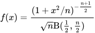
Loi de Student
f
(
x
)
=
(
1
+
x
2
/
n
)
−
n
+
1
2
n
B
(
1
2
,
n
2
)
{\displaystyle f(x)={\frac {(1+x^{2}/n)^{-{\frac {n+1}{2}}}}{{\sqrt {n}}\mathrm {B} ({\frac {1}{2}},{\frac {n}{2}})}}}
n
+
1
2
ψ
(
n
+
1
2
)
−
ψ
(
n
2
)
+
ln
n
B
(
1
2
,
n
2
)
{\displaystyle {\frac {n+1}{2}}\psi \left({\frac {n+1}{2}}\right)-\psi \left({\frac {n}{2}}\right)+\ln {\sqrt {n}}\,\mathrm {B} \left({\frac {1}{2}},{\frac {n}{2}}\right)}
Distribution de Weibull
f
(
x
)
=
c
α
x
c
−
1
exp
(
−
x
c
α
)
{\displaystyle f(x)={\frac {c}{\alpha }}x^{c-1}\exp \left(-{\frac {x^{c}}{\alpha }}\right)}
(
c
−
1
)
γ
c
+
ln
α
1
/
c
c
+
1
{\displaystyle {\frac {(c-1)\gamma }{c}}+\ln {\frac {\alpha ^{1/c}}{c}}+1}
Loi normale multidimensionnelle
f
X
(
x
1
,
…
,
x
N
)
=
{\displaystyle f_{X}(x_{1},\dots ,x_{N})=}
1
(
2
π
)
N
/
2
|
Σ
|
1
/
2
exp
(
−
1
2
(
x
−
μ
)
⊤
Σ
−
1
(
x
−
μ
)
)
{\displaystyle {\frac {1}{(2\pi )^{N/2}\left|\Sigma \right|^{1/2}}}\exp \left(-{\frac {1}{2}}(x-\mu )^{\top }\Sigma ^{-1}(x-\mu )\right)}
1
2
ln
[
(
2
π
e
)
N
|
Σ
|
]
{\displaystyle {\frac {1}{2}}\ln \left[(2\pi {\rm {e}})^{N}|\Sigma |\right]}
(en) Thomas M. Cover et Joy A. Thomas, Elements of Information Theory , New York, Wiley, 1991 (ISBN 0-471-06259-6 , lire en ligne ↑ (en) Oldrich Vasicek , « A Test for Normality Based on Sample Entropy », Journal of the Royal Statistical Society, Series B vol. 38, no 1, 1976 , p. 54–59 (DOI 10.1111/j.2517-6161.1976.tb01566.x JSTOR 2984828 ↑ (en) A. Lazo et P. Rathie, « On the entropy of continuous probability distributions », IEEE Transactions on Information Theory vol. 24, no 1, 1978 , p. 120–122 (DOI 10.1109/TIT.1978.1055832
Voir aussi
Liens externes
Portail des mathématiques Portail de l’informatique


![{\displaystyle \mathbb {E} [(X-{\widehat {X}})^{2}]\geq {\frac {1}{2\pi {\rm {e}}}}{\rm {e}}^{2h(X)}}](./_assets_/eb734a37dd21ce173a46342d1cc64c92/a83bec4eca15f964ec5f3358863427a4d68c5488.svg)


![{\displaystyle f(x)={\frac {1}{b-a}}1\!\!1_{[a,b]}}](./_assets_/eb734a37dd21ce173a46342d1cc64c92/792f886da1565070453ea160b627f8e0bf3b86e0.svg)




![{\displaystyle {\frac {1}{2}}\ln \left[(2\pi {\rm {e}})^{N}|\Sigma |\right]}](./_assets_/eb734a37dd21ce173a46342d1cc64c92/be6ad50708fe09866888447f7a4abc7475f8d10e.svg)
 )
)
 Portail des mathématiques
  Portail de l’informatique